Deconvolution of human brain cortical layers using spatially aware NNLS

In this tutorial we will explore cell-type deconvolution using different non-spatial baseline models. For illustration purpose, we consider each cortical layer as a cell type and perform deconvolution to map layer-specific expression programs to spatial locations.

import torch
import pandas as pd
from smoother import SpatialWeightMatrix, SpatialLoss
from smoother.models.deconv import NNLS, NuSVR, DWLS, LogNormReg
from smoother.losses import kl_loss
from smoother.visualization import plot_celltype_props
import matplotlib.pyplot as plt

Load the brain cortex dataset (preprocessed)

Here the expression data is truncated to keep only the top marker genes.

# change the data directory accordingly
DATA_DIR = "./data/"

# read in log_count matrices
# spatial log-normalized count matrix, num_gene x num_spot
y_df = pd.read_csv(DATA_DIR + "DLPFC_151673_marker_log_exp.txt", sep = " ", header=0)
# per-layer reference matrix, num_gene x num_celltype
x_df = pd.read_csv(DATA_DIR + "DLPFC_151673_marker_log_exp_by_layer.txt", sep = " ", header=0)

# spatial coordinates, num_spot x 2
# here we are using 10x Visium's pixel-level coordinates
# i.e., 'pxl_col_in_fullres' and 'pxl_row_in_fullres'
coords = pd.read_csv(DATA_DIR + "DLPFC_151673_coords.txt", sep = " ", header=0)
coords = coords.loc[y_df.columns,:]

print(f"Number of genes: {y_df.shape[0]}")
print(f"Number of layers: {x_df.shape[1]}")
print(f"Number of spots: {y_df.shape[1]}")

Number of genes: 350
Number of layers: 7
Number of spots: 3639

# convert data into torch tensor
x = torch.tensor(x_df.values).float()
y = torch.tensor(y_df.values).float()

Generate the spatial loss function

By default spatial weight matrix is symmetric (a requirement for the CAR and ICAR models).

# calculate spatial weight matrix
weights = SpatialWeightMatrix()
weights.calc_weights_knn(coords, k=6)

# scale the spatial weight matrix by transcriptional similarity
weights.scale_by_expr(y, reduce='none')

# convert spatial weight into loss
# note that the covariance is improper
spatial_loss = SpatialLoss('icar', weights, rho=1)

Number of spots: 3639. Average number of neighbors per spot:  5.85.
Number of spots: 3639. Average number of neighbors per spot:  5.85.

For gradient-based optimization, it’s okay to have improper covariance. However, if you are seeking a proper prior, e.g. in a Bayesian setting or for convex optimization, simply choose a smaller scale for the loss, e.g.

spatial_loss = SpatialLoss('icar', weights, rho=0.99)

If you want to use SMA or SAR model, we recommend row-scale the spatial weight matrix first for robustness. Note the ISAR model is just the row-scaled version of SAR.

# calculate spatial weight matrix
weights = SpatialWeightMatrix()
weights.calc_weights_knn(coords, row_scale = True)

# scale the spatial weight matrix by transcriptional similarity
weights.scale_by_expr(y, reduce='none', row_scale = True)

# convert spatial weight into loss
#spatial_loss = SpatialLoss('sar', weights, rho=0.999)
spatial_loss = SpatialLoss('isar', weights, rho=0.999)
#spatial_loss = SpatialLoss('sma', weights, rho=0.999, use_sparse=False)

Number of spots: 3639. Average number of neighbors per spot:  5.85.
Number of spots: 3639. Average number of neighbors per spot:  5.85.

/Users/jysumac/Projects/Smoother/smoother/weights.py:262: UserWarning: Sparse CSR tensor support is in beta state. If you miss a functionality in the sparse tensor support, please submit a feature request to https://github.com/pytorch/pytorch/issues. (Triggered internally at /Users/runner/work/pytorch/pytorch/pytorch/aten/src/ATen/SparseCsrTensorImpl.cpp:56.)

Choose the baseline model and run deconvolution

Feel free to play around with different models and prior configurations

torch.manual_seed(20221005)

# choose deconvolution model
#model = NuSVR(nu=0.5)
#model = DWLS(nonneg=True, max_weights=4)
#model = LogNormReg()
model = NNLS()

# run deconvolution without spatial loss
model.deconv(x, y, spatial_loss=None, lambda_spatial_loss=0,
             lr=1e-3, tol=1e-6, max_epochs=-1, verbose=False)

# run deconvolution with spatial loss
model_sp = NNLS()
model_sp.deconv(x, y, spatial_loss=spatial_loss, lambda_spatial_loss=10,
                lr=1e-3, tol=1e-6, max_epochs=-1, verbose=False)

=== Time  8.10s. Total epoch 2393. Final loss: (total) 0.253. (spatial) 0.000.
=== Time  13.74s. Total epoch 2379. Final loss: (total) 0.253. (spatial) 0.000.

# compare spatial heterogeneity with and without spatial loss
kl_losses = [kl_loss(torch.nn.functional.softmax(m.get_props().T, dim=0), weights.swm.to_dense())
             for m in [model, model_sp]]

print(f"Weighted KL-loss: (NNLS): {kl_losses[0]:.4f}, (+ spatial loss): {kl_losses[1]:.4f}")

Weighted KL-loss: (NNLS): 0.0027, (+ spatial loss): 0.0005

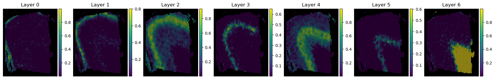
Visualize results

The regular NNLS

# extract estimated celltype abundances
ct_abundances = model.get_props()
plot_celltype_props(
    ct_abundances, coords, cell_type_names=[f'Layer {i}' for i in range(7)],
    n_col=7, figsize=[21, 3]
)

NNLS (+ spatial loss)

# extract estimated celltype abundances
ct_abundances_sp = model_sp.get_props()
plot_celltype_props(
    ct_abundances_sp, coords, cell_type_names=[f'Layer {i}' for i in range(7)],
    n_col=7, figsize=[21, 3]
)

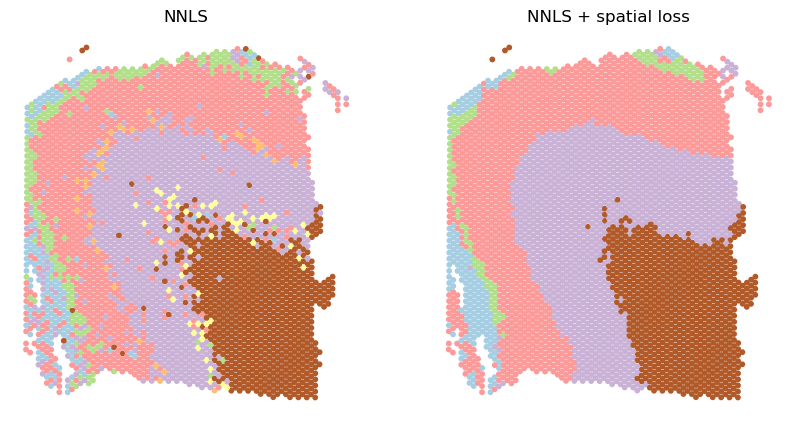
Colored by the max proportions

# colored by max coefficient
fig, (ax1, ax2)= plt.subplots(1, 2, figsize = (10, 5))
ax1.scatter(coords['pxl_col_in_fullres'], coords['pxl_row_in_fullres'],
            c = ct_abundances.argmax(1), s = 10, cmap='Paired')
ax2.scatter(coords['pxl_col_in_fullres'], coords['pxl_row_in_fullres'],
            c = ct_abundances_sp.argmax(1), s = 10, cmap='Paired')

ax1.set_title('NNLS')
ax2.set_title('NNLS + spatial loss')
ax1.axis('off')
ax2.axis('off')

plt.show()

(Optional) Solve deconvolution models using convex optimization

Before running the following example, please make sure you have the package CVXPY installed.

# calculate spatial weight matrix
weights = SpatialWeightMatrix()
weights.calc_weights_knn(coords, k=6)

# scale the spatial weight matrix by transcriptional similarity
weights.scale_by_expr(y, reduce='none')
spatial_loss = SpatialLoss('icar', weights, rho=0.99, standardize_cov=True)

# select model and run deconvolution
model = NNLS(backend='cvxpy')
#model = DWLS(backend='cvxpy', max_weights=4)
#model = NuSVR(backend='cvxpy', nonneg=True)
model.deconv(x, y, spatial_loss=None, lambda_spatial_loss=0)

#model_sp = LinearRegression(backend='cvxpy')
model_sp = NNLS(backend='cvxpy')
#model_sp = DWLS(backend='cvxpy', max_weights=4)
#model_sp = NuSVR(backend='cvxpy', nonneg=True)
model_sp.deconv(x, y, spatial_loss, lambda_spatial_loss=10)

Number of spots: 3639. Average number of neighbors per spot:  5.85.
Number of spots: 3639. Average number of neighbors per spot:  5.85.
=== Time  9.19s. Loss: (total)  0.252, (model)  0.252, (spatial)  0.000
=== Time  22.16s. Loss: (total)  0.253, (model)  0.253, (spatial)  0.001

The regular NNLS

# extract estimated celltype abundances
ct_abundances = model.get_props()
plot_celltype_props(
    ct_abundances, coords, cell_type_names=[f'Layer {i}' for i in range(7)],
    n_col=7, figsize=[21, 3]
)

NNLS (+ spatial loss)

# extract estimated celltype abundances
ct_abundances_sp = model_sp.get_props()
plot_celltype_props(
    ct_abundances_sp, coords, cell_type_names=[f'Layer {i}' for i in range(7)],
    n_col=7, figsize=[21, 3]
)

Colored by the max proportions

# colored by max coefficient
fig, (ax1, ax2)= plt.subplots(1, 2, figsize = (10, 5))
ax1.scatter(coords['pxl_col_in_fullres'], coords['pxl_row_in_fullres'],
            c = ct_abundances.argmax(1), s = 10, cmap='Paired')
ax2.scatter(coords['pxl_col_in_fullres'], coords['pxl_row_in_fullres'],
            c = ct_abundances_sp.argmax(1), s = 10, cmap='Paired')

ax1.set_title('NNLS')
ax2.set_title('NNLS + spatial loss')
ax1.axis('off')
ax2.axis('off')

plt.show()

(Optional) Solve deconvolution models using convex optimization with warm start

Warm start allows the fine-tuning of hyperparameters, in this case the smoothing strength lambda_sp

# calculate spatial weight matrix
weights = SpatialWeightMatrix()
weights.calc_weights_knn(coords, k=6)

# scale the spatial weight matrix by transcriptional similarity
weights.scale_by_expr(y, reduce='none')
spatial_loss = SpatialLoss('icar', weights, rho=0.99, standardize_cov=True)

props = []
lambda_sp_losses = [0, 1, 3, 10]

model = NNLS(backend='cvxpy', bias=True)
# if models only differ by lambda_spatial_loss,
# will enable warm start to speed up computation
for l_sp_loss in lambda_sp_losses:
    model.deconv(x, y, spatial_loss, lambda_spatial_loss=l_sp_loss)
    props.append(model.get_props())

Number of spots: 3639. Average number of neighbors per spot:  5.85.
Number of spots: 3639. Average number of neighbors per spot:  5.85.
=== Time  17.65s. Loss: (total)  0.252, (model)  0.252, (spatial)  0.000
=== Time  7.37s. Loss: (total)  0.252, (model)  0.252, (spatial)  0.000
=== Time  7.37s. Loss: (total)  0.253, (model)  0.252, (spatial)  0.000
=== Time  10.49s. Loss: (total)  0.253, (model)  0.253, (spatial)  0.001

# visualization
# colored by coefficients layer-by-layer
fig, axes = plt.subplots(4, 7, figsize = (16, 10))
for i in range(7):
    for j, l_sp_loss in enumerate(lambda_sp_losses):
        axes[j][i].scatter(coords['pxl_col_in_fullres'], coords['pxl_row_in_fullres'],
                           c = props[j][:, i], s = 1)

    axes[0][i].set_title(f"Layer {i}")

for ax in axes.flatten():
    ax.set_xticks([])
    ax.set_yticks([])

for j, l_sp_loss in enumerate(lambda_sp_losses):
    axes[j][0].set_ylabel(f'NNLS + lsp_{l_sp_loss}')

plt.show()