Data imputation using a hidden Markov random field with the spatial prior

In this tutorial we will explore data imputation and resolution enhancement. In a nutshell, Smoother assumes that the observation is generated by a hidden Gaussian Markov random field whose mean at each spot follows a zero-centered MVN prior defined by spatial coordinates.

\[Y_{obs} | \mu \sim \mathcal{N}(\mu,\,\sigma^{2}), \quad \mu \sim \text{MVN}(0,\,\Sigma)\]

import torch
import numpy as np
import pandas as pd
from smoother import SpatialWeightMatrix, SpatialLoss
from smoother.models.impute import ImputeTorch
import matplotlib.pyplot as plt
import scipy

Load the brain cortex dataset (preprocessed)

Here the expression data is truncated to keep only the top marker genes.

# change the data directory accordingly
DATA_DIR = "./data/"

# read in log_count matrices
# spatial log-normalized count matrix, num_gene x num_spot
y_df = pd.read_csv(DATA_DIR + "DLPFC_151673_marker_log_exp.txt", sep = " ", header=0)

# spatial coordinates, num_spot x 2
# here we are using 10x Visium's pixel-level coordinates
# i.e., 'pxl_col_in_fullres' and 'pxl_row_in_fullres'
coords = pd.read_csv(DATA_DIR + "DLPFC_151673_coords.txt", sep = " ", header=0)
coords = coords.loc[y_df.columns,:]

print(f"Number of genes: {y_df.shape[0]}")
print(f"Number of spots: {y_df.shape[1]}")

Number of genes: 350
Number of spots: 3639

# convert expression data into torch tensor
y = torch.tensor(y_df.values).float()

Generate the spatial loss function

By default spatial weight matrix is symmetric (a requirement for the CAR and ICAR models).

# calculate spatial weight matrix
weights = SpatialWeightMatrix()
weights.calc_weights_knn(coords, k=6)

# scale the spatial weight matrix by transcriptional similarity
weights.scale_by_expr(y)

# convert spatial weight into loss
spatial_loss = SpatialLoss('icar', weights, rho=0.99, standardize_cov=True)

Number of spots: 3639. Average number of neighbors per spot:  5.85.

Data imputation using pytorch-based implementations

ImputeTorch essentially maximize the log likelihood using gradient ascent.

Smooth gene expression at observed locations

In the first scenario, we consider the recovery of the underlying true expression of selected marker genes. Note that each variable (gene) is considered independent and optimized individually.

# select genes to smooth
ft_ind = [110,209,250,308,35]
y_obs = y[ft_ind,:].T # 5 x num_spots

# run imputation
m = ImputeTorch(y_obs, spatial_loss, fixed_obs = False, nonneg=True, lambda_spatial_loss = 1,
                 verbose = False, lr = 1e-1, max_epochs = -1, tol = 1e-8)
y_imp = m.get_results()

=== Time  0.11s. Total epoch 120. Final loss: (total)  0.303. (spatial)  0.148.

fig, axs = plt.subplots(ncols=len(ft_ind), nrows = 2, figsize = [3*len(ft_ind), 3*2])
for i, ax_col in enumerate(axs.T):
    ax_col[0].scatter(coords['pxl_col_in_fullres'], coords['pxl_row_in_fullres'],
                      c = y_obs[:,i], s = 3)
    ax_col[1].scatter(coords['pxl_col_in_fullres'], coords['pxl_row_in_fullres'],
                      c = y_imp[:,i], s = 3)

    if i == 0:
        ax_col[0].set_ylabel('Raw')
        ax_col[1].set_ylabel('Smoothed')

for ax in axs.flatten():
    ax.set_facecolor('black')
    ax.set_xticks([])
    ax.set_yticks([])

plt.show()

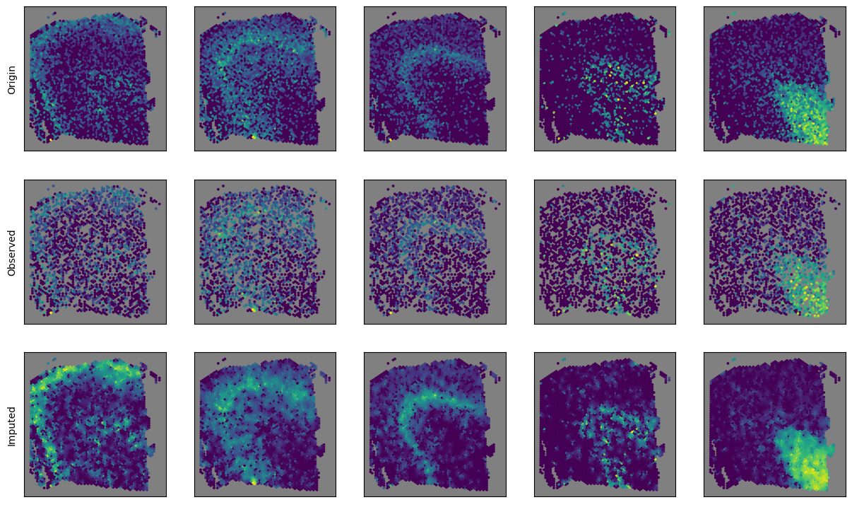
Impute expression at unseen locations while fixing the observed

In the second scenario, we consider the imputation of expression at new locations using information from the neighbors. Note that the spatial prior is constructed based on coordinates of all spots (observed + missing). For resolution enhancement purpose, simply concatenate the query coordinates to coords and reconstruct the spatial loss function before running the imputation model.

# select genes to smooth
ft_ind = [110,209,250,308,35]

# select spots to mask out
obs_ind = np.arange(2000) # observed spots
ms_ind = [i for i in range(y.shape[1]) if i not in obs_ind] # missing spots
y_orig = y[ft_ind, :].T
y_obs = y[ft_ind, :][:, obs_ind].T
y_ms = y[ft_ind, :][:, ms_ind].T

# run imputation
m = ImputeTorch(y_obs, spatial_loss, fixed_obs = True, nonneg=True, lambda_spatial_loss = 1,
                lr = 1e-2, tol = 1e-8, max_epochs = -1, verbose = False)
y_imp = m.get_results()

=== Time  0.39s. Total epoch 568. Final loss: (total)  0.368. (spatial)  0.368.

fig, axs = plt.subplots(ncols=len(ft_ind), nrows = 3, figsize = [3*len(ft_ind), 3*3])
for i, ax_col in enumerate(axs.T):
    ax_col[0].scatter(coords['pxl_col_in_fullres'], coords['pxl_row_in_fullres'],
                      c = y_orig[:,i], s = 3)
    ax_col[1].scatter(coords['pxl_col_in_fullres'][obs_ind], coords['pxl_row_in_fullres'][obs_ind],
                      c = y_obs[:,i], s = 3)
    ax_col[2].scatter(coords['pxl_col_in_fullres'], coords['pxl_row_in_fullres'],
                      c = y_imp[:,i], s = 3)

    if i == 0:
        ax_col[0].set_ylabel('Origin')
        ax_col[1].set_ylabel('Observed')
        ax_col[2].set_ylabel('Imputed')

for ax in axs.flatten():
    ax.set_facecolor('gray')
    ax.set_xticks([])
    ax.set_yticks([])

plt.show()

fig, axs = plt.subplots(ncols=len(ft_ind), nrows = 2, figsize = [3*len(ft_ind), 3*2])
for i, ax_col in enumerate(axs.T):
    ax_col[0].scatter(y_obs[:,i], y_imp[obs_ind,i], s = 2, alpha = 0.2)
    ax_col[0].set_title(f"R = {scipy.stats.pearsonr(y_obs[:,i].T, y_imp[obs_ind,i].T)[0]:.3f}\n"+
                        f"p = {scipy.stats.pearsonr(y_obs[:,i].T, y_imp[obs_ind,i].T)[1]:.3f}")
    ax_col[1].scatter(y_ms[:,i], y_imp[ms_ind,i], s = 2, alpha = 0.2)
    ax_col[1].set_title(f"R = {scipy.stats.pearsonr(y_ms[:,i].T, y_imp[ms_ind,i].T)[0]:.3f}\n"+
                        f"p = {scipy.stats.pearsonr(y_ms[:,i].T, y_imp[ms_ind,i].T)[1]:.3f}")

    if i == 0:
        ax_col[0].set_ylabel('Observed')
        ax_col[1].set_ylabel('Missing')

for ax in axs.flatten():
    ax.set_xlabel('True value')

plt.tight_layout()
plt.show()

/var/folders/_f/m4v2g8c54gdfks59bp2f2cm80000gn/T/ipykernel_15237/515326798.py:4: UserWarning: The use of `x.T` on tensors of dimension other than 2 to reverse their shape is deprecated and it will throw an error in a future release. Consider `x.mT` to transpose batches of matricesor `x.permute(*torch.arange(x.ndim - 1, -1, -1))` to reverse the dimensions of a tensor. (Triggered internally at  /Users/runner/miniforge3/conda-bld/pytorch-recipe_1664817728005/work/aten/src/ATen/native/TensorShape.cpp:2985.)
  ax_col[0].set_title(f"R = {scipy.stats.pearsonr(y_obs[:,i].T, y_imp[obs_ind,i].T)[0]:.3f}\n"+

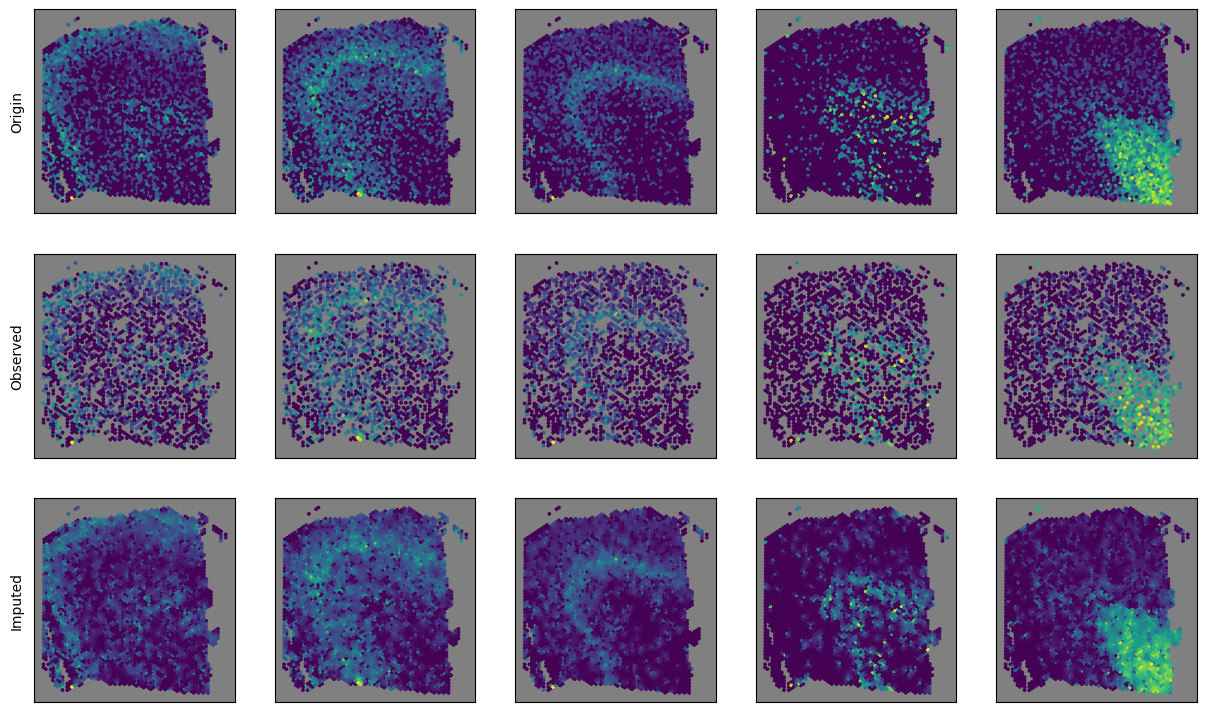
Impute expression at unseen and the observed locations

In the third scenario, we consider the imputation of expression at all locations. The observed expression values can also be updated to enforce spatial coherence, similar to the first scenario.

# select genes to smooth
ft_ind = [110,209,250,308,35]

# select spots to mask out
obs_ind = np.arange(2000) # observed spots
ms_ind = [i for i in range(y.shape[1]) if i not in obs_ind] # missing spots
y_orig = y[ft_ind, :].T
y_obs = y[ft_ind, :][:, obs_ind].T
y_ms = y[ft_ind, :][:, ms_ind].T


# run imputation
m = ImputeTorch(y_obs, spatial_loss, fixed_obs = False, nonneg=True, lambda_spatial_loss = 1,
                lr = 1e-2, tol = 1e-8, max_epochs = -1, verbose = False)
y_imp = m.get_results()

=== Time  0.58s. Total epoch 724. Final loss: (total)  0.211. (spatial)  0.131.

fig, axs = plt.subplots(ncols=len(ft_ind), nrows = 3, figsize = [3*len(ft_ind), 3*3])
for i, ax_col in enumerate(axs.T):
    ax_col[0].scatter(coords['pxl_col_in_fullres'], coords['pxl_row_in_fullres'],
                      c = y_orig[:,i], s = 3)
    ax_col[1].scatter(coords['pxl_col_in_fullres'][obs_ind], coords['pxl_row_in_fullres'][obs_ind],
                      c = y_obs[:,i], s = 3)
    ax_col[2].scatter(coords['pxl_col_in_fullres'], coords['pxl_row_in_fullres'],
                      c = y_imp[:,i], s = 3)

    if i == 0:
        ax_col[0].set_ylabel('Origin')
        ax_col[1].set_ylabel('Observed')
        ax_col[2].set_ylabel('Imputed')

for ax in axs.flatten():
    ax.set_facecolor('gray')
    ax.set_xticks([])
    ax.set_yticks([])

plt.show()

fig, axs = plt.subplots(ncols=len(ft_ind), nrows = 2, figsize = [3*len(ft_ind), 3*2])
for i, ax_col in enumerate(axs.T):
    ax_col[0].scatter(y_obs[:,i], y_imp[obs_ind,i], s = 2, alpha = 0.2)
    ax_col[0].set_title(f"R = {scipy.stats.pearsonr(y_obs[:,i].T, y_imp[obs_ind,i].T)[0]:.3f}\n"+
                        f"p = {scipy.stats.pearsonr(y_obs[:,i].T, y_imp[obs_ind,i].T)[1]:.3f}")
    ax_col[1].scatter(y_ms[:,i], y_imp[ms_ind,i], s = 2, alpha = 0.2)
    ax_col[1].set_title(f"R = {scipy.stats.pearsonr(y_ms[:,i].T, y_imp[ms_ind,i].T)[0]:.3f}\n"+
                        f"p = {scipy.stats.pearsonr(y_ms[:,i].T, y_imp[ms_ind,i].T)[1]:.3f}")

    if i == 0:
        ax_col[0].set_ylabel('Observed')
        ax_col[1].set_ylabel('Missing')

for ax in axs.flatten():
    ax.set_xlabel('True value')

plt.tight_layout()
plt.show()

(Optional) Data imputation using CVXPY-based implementations

Since the SpatialLoss is quadratic wrt the variable of interest, the imputation problem can be solved by convex optimization, which is what ImputeConvex does. This would require the installation of the cvxpy package. In general, CVXPY-based imputation is more accurate but slightly slower. When the number of genes to impute is large, CVXPY may encounter numeric issues.

# please make sure cvxpy is installed
from smoother.models.impute import ImputeConvex

Smooth gene expression at observed locations

# select genes to smooth
ft_ind = [110,209,250,308,35]

y_obs = y[ft_ind,:].T

# run imputation
m = ImputeConvex(y_obs, spatial_loss, fixed_obs = False, nonneg=True, lambda_spatial_loss = 1)
y_imp = m.get_results()

=== Time  0.23s. Loss: (total)  0.220, (recon)  0.139, (spatial)  0.082

fig, axs = plt.subplots(ncols=len(ft_ind), nrows = 2, figsize = [3*len(ft_ind), 3*2])
for i, ax_col in enumerate(axs.T):
    ax_col[0].scatter(coords['pxl_col_in_fullres'], coords['pxl_row_in_fullres'],
                      c = y_obs[:,i], s = 3)
    ax_col[1].scatter(coords['pxl_col_in_fullres'], coords['pxl_row_in_fullres'],
                      c = y_imp[:,i], s = 3)

    if i == 0:
        ax_col[0].set_ylabel('Raw')
        ax_col[1].set_ylabel('Smoothed')

for ax in axs.flatten():
    ax.set_facecolor('black')
    ax.set_xticks([])
    ax.set_yticks([])

plt.show()

Impute expression at unseen locations while fixing the observed

# select genes to smooth
ft_ind = [110,209,250,308,35]

# select spots to mask out
obs_ind = np.arange(2000) # observed spots
ms_ind = [i for i in range(y.shape[1]) if i not in obs_ind] # missing spots
y_orig = y[ft_ind, :].T
y_obs = y[ft_ind, :][:, obs_ind].T
y_ms = y[ft_ind, :][:, ms_ind].T

# run imputation
m = ImputeConvex(y_obs, spatial_loss, fixed_obs = True, nonneg=True, lambda_spatial_loss = 1)
y_imp = m.get_results()

=== Time  0.16s. Loss: (total)  0.368, (recon)  0.000, (spatial)  0.368

fig, axs = plt.subplots(ncols=len(ft_ind), nrows = 3, figsize = [3*len(ft_ind), 3*3])
for i, ax_col in enumerate(axs.T):
    ax_col[0].scatter(coords['pxl_col_in_fullres'], coords['pxl_row_in_fullres'],
                      c = y_orig[:,i], s = 3)
    ax_col[1].scatter(coords['pxl_col_in_fullres'][obs_ind], coords['pxl_row_in_fullres'][obs_ind],
                      c = y_obs[:,i], s = 3)
    ax_col[2].scatter(coords['pxl_col_in_fullres'], coords['pxl_row_in_fullres'],
                      c = y_imp[:,i], s = 3)

    if i == 0:
        ax_col[0].set_ylabel('Origin')
        ax_col[1].set_ylabel('Observed')
        ax_col[2].set_ylabel('Imputed')

for ax in axs.flatten():
    ax.set_facecolor('gray')
    ax.set_xticks([])
    ax.set_yticks([])

plt.show()

fig, axs = plt.subplots(ncols=len(ft_ind), nrows = 2, figsize = [3*len(ft_ind), 3*2])
for i, ax_col in enumerate(axs.T):
    ax_col[0].scatter(y_obs[:,i], y_imp[obs_ind,i], s = 2, alpha = 0.2)
    ax_col[0].set_title(f"R = {scipy.stats.pearsonr(y_obs[:,i].T, y_imp[obs_ind,i].T)[0]:.3f}\n"+
                        f"p = {scipy.stats.pearsonr(y_obs[:,i].T, y_imp[obs_ind,i].T)[1]:.3f}")
    ax_col[1].scatter(y_ms[:,i], y_imp[ms_ind,i], s = 2, alpha = 0.2)
    ax_col[1].set_title(f"R = {scipy.stats.pearsonr(y_ms[:,i].T, y_imp[ms_ind,i].T)[0]:.3f}\n"+
                        f"p = {scipy.stats.pearsonr(y_ms[:,i].T, y_imp[ms_ind,i].T)[1]:.3f}")

    if i == 0:
        ax_col[0].set_ylabel('Observed')
        ax_col[1].set_ylabel('Missing')

for ax in axs.flatten():
    ax.set_xlabel('True value')

plt.tight_layout()
plt.show()

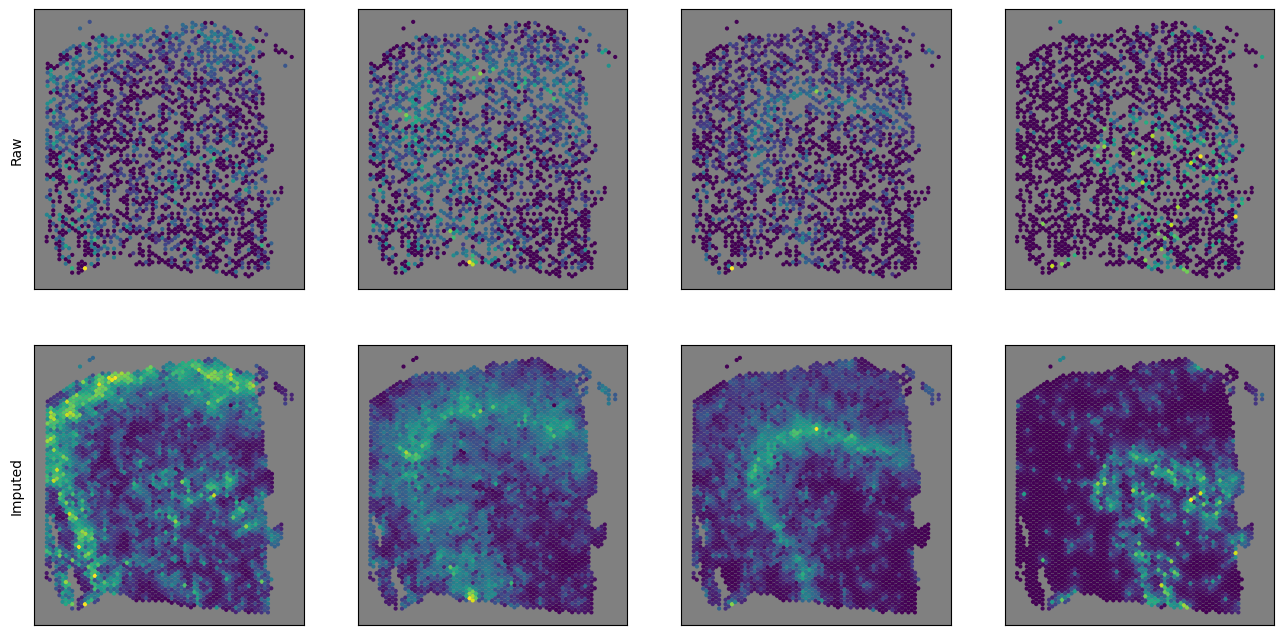
Impute expression at unseen and the observed locations

# select genes to smooth
ft_ind = [110,209,250,308]

# select spots to mask out
obs_ind = np.arange(2000) # observed spots
ms_ind = [i for i in range(y.shape[1]) if i not in obs_ind] # missing spots
y_orig = y[ft_ind, :].T
y_obs = y[ft_ind, :][:, obs_ind].T
y_ms = y[ft_ind, :][:, ms_ind].T

# run imputation
m = ImputeConvex(y_obs, spatial_loss, fixed_obs = False, nonneg=True, lambda_spatial_loss = 1)
y_imp = m.get_results()

=== Time  0.17s. Loss: (total)  0.173, (recon)  0.085, (spatial)  0.088

fig, axs = plt.subplots(ncols=len(ft_ind), nrows = 2, figsize = [4*len(ft_ind), 4*2])
for i, ax_col in enumerate(axs.T):
    ax_col[0].scatter(coords['pxl_col_in_fullres'][obs_ind], coords['pxl_row_in_fullres'][obs_ind],
                      c = y_obs[:,i], s = 4)
    ax_col[1].scatter(coords['pxl_col_in_fullres'], coords['pxl_row_in_fullres'],
                      c = y_imp[:,i], s = 4)

    if i == 0:
        ax_col[0].set_ylabel('Raw')
        ax_col[1].set_ylabel('Imputed')

for ax in axs.flatten():
    ax.set_facecolor('gray')
    ax.set_xticks([])
    ax.set_yticks([])

plt.show()

fig, axs = plt.subplots(ncols=len(ft_ind), nrows = 2, figsize = [3*len(ft_ind), 3*2])
for i, ax_col in enumerate(axs.T):
    ax_col[0].scatter(y_obs[:,i], y_imp[obs_ind,i], s = 2, alpha = 0.2)
    ax_col[0].set_title(f"R = {scipy.stats.pearsonr(y_obs[:,i].T, y_imp[obs_ind,i].T)[0]:.3f}\n"+
                        f"p = {scipy.stats.pearsonr(y_obs[:,i].T, y_imp[obs_ind,i].T)[1]:.3f}")
    ax_col[1].scatter(y_ms[:,i], y_imp[ms_ind,i], s = 2, alpha = 0.2)
    ax_col[1].set_title(f"R = {scipy.stats.pearsonr(y_ms[:,i].T, y_imp[ms_ind,i].T)[0]:.3f}\n"+
                        f"p = {scipy.stats.pearsonr(y_ms[:,i].T, y_imp[ms_ind,i].T)[1]:.3f}")

    if i == 0:
        ax_col[0].set_ylabel('Observed')
        ax_col[1].set_ylabel('Missing')

for ax in axs.flatten():
    ax.set_xlabel('True value')

plt.tight_layout()
plt.show()